
Select projects | see all
-
 Descriptionclose
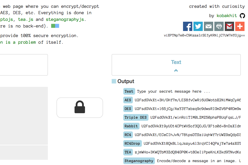
eикrуpт, inspired by cryptii, is a web page where you can encrypt/decrypt messages using algorythms such as AES, DES, etc. Everything is done in your browser using javascript, cryptojs, tea.js and steganographyjs. Nothing is send to the server (there is no back-end). This tool got viral on reddit.
Recent Activity | see all
Blog | Latest posts
-
Ubuntu 16.04 alongside Windows 7/8/10 for Data Science
beginner #python #jupyter #linux #windows #r #data-science #git #anacondaHaving a Lenovo Y500 laptop with good specs (8GB RAM, 4 processors) that runs on Windows 7 made me feel limited when it came to scientific computing. Unix based systems like Linux and Mac OS are more convenient to use than Windows systems. As a result, after doing some research I decided to install a Linux distribution Ubuntu 16.04 aka Xenial alongside my Widnows 7 OS. This gives me the option to boot any of the two. I heavily use Python 2.7, 3.5 and R which I all install on my new Ubuntu partition. Below are the steps that worked for me. Hopefully, you find them useful.
Tabe of contents
- Dual Boot Windows 7/8/10 and Ubuntu 16.04 Xenial
- Install R
- Install Rstudio
- Install Git
- Install Python 2.7 and 3.5 (Anaconda distribution and virtual environment)
- Install Sublime Text 3
Dual Boot Windows 7/8/10 and Ubuntu 16.04 Xenial
Create Bootable USB
You will need to have
- Ubuntu 16.04 ISO
- Rufus to create a bootable USB Device
- A USB device with at least 8GB space
You can start with burning the Ubuntu ISO onto the USB drive using Rufus. Just launch Rufus choose the ISO, the USB drive and press the start button. Now, you have a bootable USB drive with Ubuntu 16.04.
Partition Hard Drive
Now, we need to create free space on the HD for the Ubuntu 16.04 to be installed on. There are a lot of guides online and I present the way that worked for me. I use the Windows default app
diskmgmt.msc. Just search for it and launch it. Choose the hard disk with the most free space on it. Right click on it and choose shrink option. You only have to shrink it by 20GB. It is enough for Ubuntu 16.04 and 18GB of storage for your files. You can go above 20GB of course. That’s it. At this point we can boot Ubuntu Xenial and install it if we like it.Boot from USB and Install
Whatever laptop you have bring up the boot menu on startup. For me (Lenovo Y500) there is a button on the left behind the power plug. In the boot menu you should see an option for a USB drive. Boot from the USB and you will see
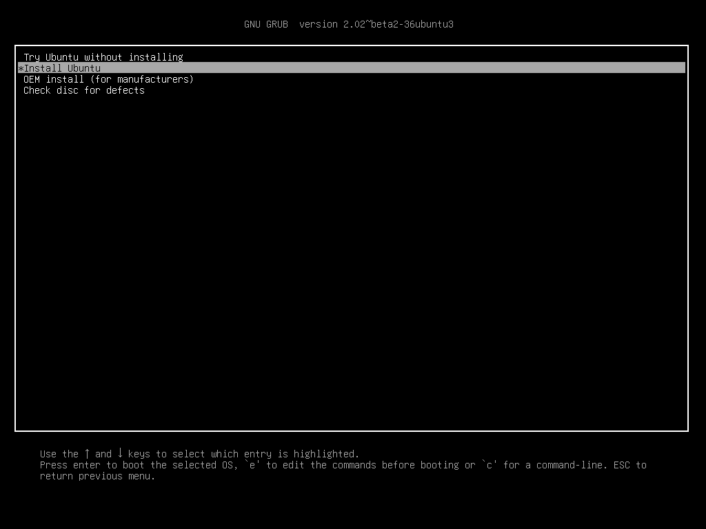
You can try Ubuntu Xenial out first by going with the first option (Try Ubuntu without installing). Once you are convinced it is great (more convenient than Windows for data purposes at least), shutdown, boot from USB again and install it. At some point you will see this

Normally, after you shrank one of your partitions and allocated free space of 20GB or above there should also be an option Install alongside Windows. If you do not see it after going through previous steps let me know and I will look into it.
Finally, once installed run in terminal
sudo update-grubThis will update the boot loader menu and nexxt time you see boot menu you will be able to choose Ubuntu or Windows. Lets move on to installing statistical software.
Install R
To install R on Ubuntu 16.04 aka Xenial execute the below commands in terminal.
sudo add-apt-repository ppa:marutter/rrutter
sudo apt-get update
sudo apt-get install r-base r-base-dev
Install Rstudio
Now, that we have R installed lets get Rstudio.
sudo apt-get install gdebi-core
wget https://download1.rstudio.org/rstudio-0.99.902-amd64.deb
sudo gdebi -n rstudio-0.99.902-amd64.deb
rm rstudio-0.99.902-amd64.deb
Install Git
sudo apt-get install gitInstall Python 2.7 and 3.5 (Anaconda distribution and virtual environment)
We will install Anaconda 2.3 Python distibution and then create a virtual Python 3.5 environment using
conda.Instal Anaconda Python 2.7
First, install Anaconda 2.3 which is based on Python 2.7 .
wget https://3230d63b5fc54e62148e-c95ac804525aac4b6dba79b00b39d1d3.ssl.cf1.rackcdn.com/Anaconda-2.3.0-Linux-x86_64.sh

bash Anaconda-2.3.0-Linux-x86_64.sh
rm Anaconda-2.3.0-Linux-x86_64.sh
You will be promted to read the user agreement and set some parameters during installation. Go through it and once the installation is finished run below commands and you will see something like this.
koba@kobakhit:~$ exec bash
koba@kobakhit:~$ python
Python 2.7.10 |Anaconda 2.3.0 (64-bit)| (default, May 28 2015, 17:02:03)
[GCC 4.4.7 20120313 (Red Hat 4.4.7-1)] on linux2
Type "help", "copyright", "credits" or "license" for more information.
Anaconda is brought to you by Continuum Analytics.
Please check out: http://continuum.io/thanks and https://binstar.org
>>> exit()
Type
exit()and enter to get back to bash.Install Anaconda Python 3.5 virtual environment
Anaconda is installed and is the default python executable. Second, lets create Python 3.5 virtual environment. Below info is taken from a concise cookboook.
To install a virtual python environment you want use this command template
conda create -n yourenvname python=x.x anaconda. For example, I created a virtual python 3.5 environment calledtpot. For a list of available python versions typeconda search "^python$".conda create -n tpot python=3.5 anacondaTo activate and deactivate your virtual environment type
source activate tpot
source deactivate tpot

# remove a virtual enironment
conda remove -n tpot -all
Now, you have Python versions 2.7 and 3.5 with all the Numpy, Scikit-Learn, Pandas, etc. packages already installed thanks to Anaconda distribution. As a finishing touch lets install jupyter to work with IPython notebooks.
conda install jupyterYou will have to install one for your virtual environment as well. Recall, I created a virtual env called
tpotpreviously. You might need to close and reopen the terminal for thesource activateto work.source activate tpot conda install jupyter source deactivateTo start IPython run
jupyter notebookwhich will create a tab in your browser.Install Sublime Text 3
This is my choice of text editor.
sudo add-apt-repository ppa:webupd8team/sublime-text-3
sudo apt-get update
sudo apt-get install sublime-text-installer
Conclusion
There are several distros created for scietific computing that have some software preinstalled. To name a few
For software highlights of each you can refer to this article. I can promise you that none at the moment of writing had all the software I wanted installed (R and Rstudio, Anaconda Python 2.7 and 3.5). Until somebody releases a data science Linux distro Ubuntu Xenial is the most optimal choice in terms of flexibility and convenience.
Bonus
Install Jekyll (static website generator)
sudo apt-get install jekyll
...Read more -
Visualizing Indego bike geoson data in Python using Folium
beginner #python #ipynb #geoson #indego-bike-share #phillyA simple example of visualizing geoson data in python using Folium. We obtain Philly Indego bike data from opendataphilly website. We download the data using the website’s free public api.
import json,urllib2
import pandas as pd

# add a header so that the website doesnt give 403 error
opener = urllib2.build_opener()
opener.addheaders = [('User-agent', 'Mozilla/5.0')]
response = opener.open('https://api.phila.gov/bike-share-stations/v1')

# parse json using pandas
df = pd.read_json(response)
df.head()
features type 0 {u'geometry': {u'type': u'Point', u'coordinate... FeatureCollection 1 {u'geometry': {u'type': u'Point', u'coordinate... FeatureCollection 2 {u'geometry': {u'type': u'Point', u'coordinate... FeatureCollection 3 {u'geometry': {u'type': u'Point', u'coordinate... FeatureCollection 4 {u'geometry': {u'type': u'Point', u'coordinate... FeatureCollection Now,
dfis a dictionary of dictionaries. We are interested in the features column. Each entry looks like this.df['features'][0]{u'geometry': {u'coordinates': [-75.16374, 39.95378], u'type': u'Point'}, u'properties': {u'addressCity': u'Philadelphia', u'addressState': u'PA', u'addressStreet': u'1401 John F. Kennedy Blvd.', u'addressZipCode': u'19102', u'bikesAvailable': 6, u'closeTime': u'23:58:00', u'docksAvailable': 19, u'eventEnd': None, u'eventStart': None, u'isEventBased': False, u'isVirtual': False, u'kioskId': 3004, u'kioskPublicStatus': u'Active', u'name': u'Municipal Services Building Plaza', u'openTime': u'00:02:00', u'publicText': u'', u'timeZone': u'Eastern Standard Time', u'totalDocks': 25, u'trikesAvailable': 0}, u'type': u'Feature'}# number of rows (bike stations) len(df["features"])73We organize data first before plotting to follow a Folium example. Basically we need to create a list of tuples with latitude and longtitude. We called it
coordinates.# Organize data coordinates = [] for i in range(0,len(df['features'])): coordinates.append(((df["features"][i]["geometry"]['coordinates']))) # convert list of lists to list of tuples coordinates = [tuple([i[1],i[0]]) for i in coordinates] print(coordinates[0:10])[(39.95378, -75.16374), (39.94733, -75.14403), (39.9522, -75.20311), (39.94517, -75.15993), (39.98082, -75.14973), (39.95576, -75.18982), (39.94711, -75.16618), (39.96046, -75.19701), (39.94217, -75.1775), (39.96317, -75.14792)]Let’s visualize the coordinates geoson data using Folium.
import folium
import numpy as np

#print(folium.__file__)
#print(folium.__version__)

# get center of map
meanlat = np.mean([i[0] for i in coordinates])
meanlon = np.mean([i[1] for i in coordinates])

# initialize map
mapa = folium.Map(location=[meanlat, meanlon],
                  tiles='OpenStreetMap', zoom_start=13)
# add markers
for i in range(0,len(coordinates)):

    # create popup on click
    html="""
    Address: {}<br>
    Bikes available: {}<br>
    Docks: {}<br>
    """
    html = html.format(df['features'][i]['properties']['addressStreet'],\
               df['features'][i]['properties']['bikesAvailable'],\
               df['features'][i]['properties']['docksAvailable'])
    iframe = folium.element.IFrame(html=html, width=150, height=150)
    popup = folium.Popup(iframe, max_width=2650)

    #  add marker to map
    folium.Marker(coordinates[i],
                  popup=popup,
                 ).add_to(mapa)

mapa # show map
We can cluster nearby points. Also, let’s look at a different background by changing the tiles argument. List of available tiles can be found in Folium github repo.
from folium.plugins import MarkerCluster # for marker clusters

# initialize map
mapa = folium.Map(location=[meanlat, meanlon],
                  tiles='Cartodb Positron', zoom_start=13)

# add marker clusters
mapa.add_children(MarkerCluster(locations=coordinates, popups=coordinates))
mapa
We can utilize Folium plugins to view the geoson data in different ways. For example, let’s generate a heat map of the bike stations in Philly. We can see that there are dense areas in center city and Chinatown mostly.
from folium.plugins import HeatMap

# initialize map
mapa = folium.Map(location=[meanlat, meanlon],
                  tiles='Cartodb Positron', zoom_start=13)

# add heat
mapa.add_children(HeatMap(coordinates))
mapa
For more examples go to the Folium’s examples page.
Resources used
...Read more -
Linear optimization and baseball teams
intermediate #r #opr #linear-optimization #integer #datatable #rmarkdownWe try to use Integer Linear Programming to build a perfect 25 men roster baseball team. We present our best team below which is the solution of the ILP model we built using the 2015 MLB season player data. If you understand baseball please evaluate our resulting baseball team and drop a comment, so that we know whether ILP can be used to get a decent baseball team. After the table I describe how we arrived at our solution.
Edit: The choice of statistics for our utility index is almost random. The main goal was to model the general constraints and objective function. This code allows to easily add desired statistics and extend the general case to include more sophisticated preferences, for example using the weight vector.
Prerequisites
To follow the process of us setting up the ILP model you should have familitarity with
- Linear algebra
- Linear optimization
- Integer programming
Data preprocessing
Let’s read in the 2015 regular season player level data.
dat = read.csv("Baseball Data.csv")
head(dat[,1:4])
## Salary Name POS Bats ## 1 510000 Joc Pederson OF L ## 2 512500 Stephen Vogt 1B L ## 3 3550000 Wilson Ramos C R ## 4 31000000 Clayton Kershaw SP ## 5 15000000 Jhonny Peralta SS R ## 6 2000000 Carlos Villanueva RelieverThe dataset has 199 rows (players). There were
NA'sfor some players and their game statistics which we replaced with 0. The reason we replaced the missing data with zeros is that when we construct the player utility index missing data won’t count towards or against players.dat[is.na(dat)] = 0Each baseball player has game statistics associated with them. Below is the list of player level data.
names(dat)## [1] "Salary" "Name" "POS" "Bats" "Throws" "Team" ## [7] "G" "PA" "HR" "R" "RBI" "SB" ## [13] "BB." "K." "ISO" "BABIP" "AVG" "OBP" ## [19] "SLG" "wOBA" "wRC." "BsR" "Off" "Def" ## [25] "WAR" "playerid"You can see the statistics description in the collapsible list below or appendix.
-
Baseball statistics abbreviations
- PA - Plate appearance: number of completed batting appearances
- HR - Home runs: hits on which the batter successfully touched all four bases, without the contribution of a fielding error
- R - Runs scored: number of times a player crosses home plate
- RBI - Run batted in: number of runners who score due to a batters’ action, except when batter grounded into double play or reached on an error
- SB - Stolen base: number of bases advanced by the runner while the ball is in the possession of the defense
- ISO - Isolated power: a hitter’s ability to hit for extra bases, calculated by subtracting batting average from slugging percentage
- BABIP - Batting average on balls in play: frequency at which a batter reaches a base after putting the ball in the field of play. Also a pitching category
- AVG - Batting average (also abbreviated BA): hits divided by at bats
- OBP - On-base percentage: times reached base divided by at bats plus walks plus hit by pitch plus sacrifice flies
- SLG - Slugging average: total bases achieved on hits divided by at-bats
- wOBA - Some argue that the OPS, on-base plus slugging, formula is flawed and that more weight should be shifted towards OBP (on-base percentage). The statistic wOBA (weighted on-base average) attempts to correct for this.
- wRC. - Weighted Runs Created (wRC): an improved version of Bill James’ Runs Created statistic, which attempted to quantify a player’s total offensive value and measure it by runs.
- BsR - Base Runs: Another run estimator, like Runs Created; a favorite of writer Tom Tango
- WAR - Wins above replacement: a non-standard formula to calculate the number of wins a player contributes to his team over a “replacement-level player”
- Off - total runs above or below average based on offensive contributions (both batting and baserunning)
- Def - total runs above or below average based on defensive contributions (fielding and position).
Since the game statistics are in different units we standardize the data by subtracting the mean and dividing by the standard deviation, $x_{changed} = \frac{x-\mu}{s}$. Additionaly, we add two new variables
Off.normandDef.normwhich are normalizedOffandDefratings using the formula $x_{changed}=\frac{x-min(x)}{max(x)-min(x)}$. We use the normalized offensive and defensive ratings to quickly evaluate the optimal team according to the ILP.# select numeric columns and relevant variables dat.scaled = scale(dat[,sapply(dat, class) == "numeric"][,c(-1:-2,-19)]) # normalize Off and Def dat$Off.norm = (dat$Off-min(dat$Off))/(max(dat$Off)-min(dat$Off)) dat$Def.norm = (dat$Def-min(dat$Def))/(max(dat$Def)-min(dat$Def)) head(dat.scaled[,1:4])## PA HR R RBI ## [1,] 0.9239111 1.2879067 0.7024833 0.4469482 ## [2,] 0.6851676 0.6505590 0.4831027 0.8744364 ## [3,] 0.6625837 0.4115537 0.0687172 0.7989973 ## [4,] -0.9634531 -0.7834733 -0.9306832 -0.9109555 ## [5,] 1.1013556 0.5708906 0.6293565 0.8744364 ## [6,] -0.9634531 -0.7834733 -0.9306832 -0.9109555Now that we have scaled player stats we will weigh them and add them up to obtain the player utility index $U_i$ for player $i$ to use it in the objective function.
$U_i(x) = w_{1}\text{PA}_i+w_{2}\text{HR}_i+w_{3}\text{R}_i+w_{4}\text{RBI}_i+w_{5}\text{SB}_i+w_{6}\text{ISO}_i+w_{7}\text{BABIP}_i+w_{8}\text{AVG}_i+w_{9}\text{OBP}_i+w_{10}\text{SLG}_i+w_{11}\text{wOBA}_i+w_{12}\text{wRC.}_i+w_{13}\text{BsR}_i+w_{14}\text{Off}_i+w_{15}\text{Def}_i+w_{16}\text{WAR}_i$
$\text{ for player } i \text{ where } i \in \{1,199\}$
By introducing weights we can construct the weight vector which best suits our preferences. For example, if we wanted the player utility index to value the offensive statistics like
RBImore than the defensive statistics likeDefwe would just assign a bigger weight to RBI. We decided to value each statistic equally, i.e. weights are equal.Constraint modelling
In baseball there are 25 active men roster and 40 men roster that includes the 25 men active roster. To start a new team we focus on building the perfect 25 men roster. Typically, a 25 men roster will consist of five starting pitchers (SP), seven relief pitchers (Reliever), two catchers (C), six infielders (IN), and five outfielders (OF). Current position variable
POShas more than 5 aforementioned groups. We group them in thePOS2variable by the five types SP, Reliever, C, IN, OF.position = function(x){ # given position x change x to group if(x %in% c("1B","2B","3B","SS")) x = "IN" else if(x %in% c("Closer")) x = "Reliever" else x=as.character(x) } dat$POS2 = sapply(dat$POS, position)Additionally, we will make sure that our 25 men active roster has at least one player of each of the following positions: first base (1B), second base (2B), third base (3B) and Short stop (SS).
There is no salary cap in the Major League Baseball association, but rather a threshold of 189$ million for the 40 men roster for period 2014-2016 beyond which a luxury tax applies. For the first time violators the tax is 22.5% of the amount they were over the threshold. We decided that we would allocate 178$ million for the 25 men roster.
To model the above basic constraints and an objective function we came up with the player utility index $U(x_1,x_2,…,x_n)$ which is a function of the chosen set of $n$ player game statistics, 16 in our case. In our model we maximize the sum of the player utility indices. We have 16 game statistics of interest which are
PA, HR, R, RBI, SB, ISO, BABIP, AVG, OBP, SLG, wOBA, wRC., BsR, Off, Def, WAR, Off.norm, Def.norm
Below is the resulting model.
\[\begin{align} \text{max } & \sum^{199}\_{i=1}U\_i\*x\_i \\\\ \text{s. t. } & \sum^{199}\_{i=1}x\_i = 25 \\\\ & \sum x\_{\text{SP}} \ge 5 \\\\ & \sum x\_{\text{Reliever}} \ge 7 \\\\ & \sum x\_{\text{C}} \ge 2 \\\\ & \sum x\_{\text{IN}} \ge 6 \\\\ & \sum x\_{\text{OF}} \ge 5 \\\\ & \sum x\_{\text{POS}} \ge 1 \text{ for } POS \in \\{\text{1B,2B,3B,SS}\\}\\\\ & \sum x\_{\text{LeftHandPitchers}} \ge 2 \\\\ & \sum x\_{\text{LeftHandBatters}} \ge 2 \\\\ & \frac{1}{25} \sum Stat\_{ij}x\_{i} \ge mean(Stat\_{j}) \text{ for } j = 1,2,...,16 \\\\ & \sum^{199}\_{i=1}salary\_i\*x\_i \le 178 \end{align}\]where
- $U_i$- utility index for player $i$, $i \in \{1,199\}$
- $x_i$ - a binary variable which is one if player $i$ is selected
- $x_{\text{SP}}, x_{\text{Reliever}}$, etc. - binary variables that are one if player $i$ has the specified attribute such as Starting pitcher (SP), left hand pitcher, etc.
- $x_{\text{POS}}$ - binary variable which is one if player $i$ plays the position $POS$, $POS \in \{\text{1B,2B,3B,SS}\}$
- $Stat_{ij}$ - game statistic $j$ for player $i$, $j \in \{1,16\}$
- $mean(Stat_{j})$ - the average of the statistic $j$ across all players
- $salary_i$ - salary for player $i$ in dollars
Constraint (2) ensures that we get 25 players. Constraints (3) through (10) ensure that number of players with certain attributes meets the required minimum. Collection of constraints (11) makes sure that our team’s average game stastistics outperform the average game statistics across all players. Constraint (12) ensures that we stay within our budget including the luxury tax.
Below is the solution of this programm.
library("lpSolve")

i = 199 # number of players (variables)

# constraints
cons = rbind(
  rep(1,i), # 25 man constraint (2)
  sapply(dat$POS2, function(x) if (x == "SP") x=1 else x=0), # (3)
  sapply(dat$POS2, function(x) if (x == "Reliever") x=1 else x=0), # (4)
  sapply(dat$POS2, function(x) if (x == "C") x=1 else x=0), # (5)
  sapply(dat$POS2, function(x) if (x == "IN") x=1 else x=0), # (6)
  sapply(dat$POS2, function(x) if (x == "OF") x=1 else x=0), # (7)
  sapply(dat$POS, function(x) if (x == "1B") x=1 else x=0), # (8)
  sapply(dat$POS, function(x) if (x == "2B") x=1 else x=0), # (8)
  sapply(dat$POS, function(x) if (x == "3B") x=1 else x=0), # (8)
  sapply(dat$POS, function(x) if (x == "SS") x=1 else x=0), # (8)
  sapply(dat$Throws, function(x) if (x == "L") x=1 else x=0), # (9)
  sapply(dat$Bats, function(x) if (x == "L") x=1 else x=0), # (10)
  t(dat[,colnames(dat.scaled)])/25, # (11) outperform the average
  dat$Salary/1000000 # (12) budget constraint
)

# model
f.obj = apply(dat.scaled,1,sum)
f.dir = c("=",rep(">=",27),"<=")
f.rhs = c(25,5,7,2,6,5,2,2,rep(1,4),
          apply(dat[,colnames(dat.scaled)],2,mean),
          178)

model = lp("max", f.obj, cons, f.dir, f.rhs, all.bin=T,compute.sens=1)
model
## Success: the objective function is 135.6201sol = model$solution sol## [1] 0 0 0 1 0 0 0 1 0 0 0 0 0 0 0 0 0 0 0 0 0 0 0 1 0 1 0 0 1 0 0 0 0 0 0 ## [36] 0 0 0 0 0 0 0 0 0 0 0 0 0 0 0 0 0 1 1 0 0 0 0 0 0 0 1 0 0 0 0 0 0 0 0 ## [71] 1 0 0 0 0 0 0 0 0 0 0 0 1 0 0 0 1 0 0 0 0 0 0 0 0 0 0 0 0 0 0 0 0 0 0 ## [106] 0 0 1 1 0 0 0 1 0 1 0 0 0 1 0 1 0 0 0 0 0 0 0 1 0 0 0 0 0 0 0 0 0 1 0 ## [141] 0 1 1 0 0 0 0 0 0 1 0 0 0 0 0 0 0 0 0 0 0 0 1 0 0 0 0 0 0 0 0 0 0 0 0 ## [176] 1 0 0 0 0 0 0 0 0 0 0 0 0 0 0 0 0 0 1 0 0 0 0 0Let’s look at our ideal baseball team given the constraints outlined above.
# selected players
dat[which(sol>0),c(1:3,6,28:29)]
## Salary Name POS Team Def.norm POS2 ## 4 31000000 Clayton Kershaw SP 0.3713163 SP ## 8 6083333 Mike Trout OF Angels 0.4125737 OF ## 24 19750000 David Price SP 0.3713163 SP ## 26 507500 Dellin Betances Closer Yankees 0.3713163 Reliever ## 29 509000 Matt Duffy 2B Giants 0.5972495 IN ## 53 17142857 Max Scherzer SP 0.3713163 SP ## 54 17277777 Buster Posey C Giants 0.5324165 C ## 62 509500 Carson Smith Closer Mariners 0.3713163 Reliever ## 71 519500 A.J. Pollock OF Diamondbacks 0.5422397 OF ## 83 535000 Trevor Rosenthal Closer Cardinals 0.3713163 Reliever ## 87 547100 Cody Allen Closer Indians 0.3713163 Reliever ## 108 2500000 Dee Gordon 2B Marlins 0.5402750 IN ## 109 2500000 Bryce Harper OF Nationals 0.2043222 OF ## 113 2725000 Lorenzo Cain OF Royals 0.6797642 OF ## 115 3083333 Paul Goldschmidt 1B Diamondbacks 0.2357564 IN ## 119 3200000 Zach Britton Closer Orioles 0.3713163 Reliever ## 121 3630000 Jake Arrieta SP 0.3713163 SP ## 129 4300000 Josh Donaldson 3B Blue Jays 0.5815324 IN ## 139 6000000 Chris Sale SP 0.3713163 SP ## 142 7000000 Russell Martin C Blue Jays 0.6110020 C ## 143 7000000 Wade Davis Closer Royals 0.3713163 Reliever ## 150 8050000 Aroldis Chapman Closer Reds 0.3713163 Reliever ## 163 10500000 Yoenis Cespedes OF - - - 0.5795678 OF ## 176 14000000 Joey Votto 1B Reds 0.1886051 IN ## 194 543000 Xander Bogaerts SS Red Sox 0.5284872 INSeems like a decent team with the mean normalized offensive and defensive ratings of 0.414495 and 0.4275835 respectively. For comparison mean normalized offensive and defensive ratings for all players are 0.3019702 and 0.3821564 respectively. Our team outperforms the average and its mean offensive and defensive ratings are better than $82.9145729$% and $78.3919598$% of other players correspondingly.

While this is a straightforward way to model the selection of the players there are several nuances we need to address. One of them is that the standardized game statistics are not additively independent. As a result, our utility index poorly measures the player’s value and is biased. It is possible to construct an unbiased utility index which has been done a lot in baseball (look up sabermetrics).
OffandDefand a lot of other statistics are examples of utility indices. A reddit user suggested a solid way to construct the utility index.Another issue we need to addrees is when we substituted the missing values with zero. Players with missing game statistics values have their utility index diminished because one of the stats used to calculate it is zero. However, imputing with zero is better than imputing with the mean in our case. By imputing with the mean we would introduce new information into the data which may be misleading, ex. g. a player’s game stat is worse/better than the average. As a result, the player utility index would be overestimated/underestimated.
Finally, I believe that using statistical and mathematical methods is only acceptable as a supplement to the decision making process not only in baseball, but in every field.
Appendix
Baseball statistics abbreviations
- PA - Plate appearance: number of completed batting appearances
- HR - Home runs: hits on which the batter successfully touched all four bases, without the contribution of a fielding error
- R - Runs scored: number of times a player crosses home plate
- RBI - Run batted in: number of runners who score due to a batters’ action, except when batter grounded into double play or reached on an error
- SB - Stolen base: number of bases advanced by the runner while the ball is in the possession of the defense
- ISO - Isolated power: a hitter’s ability to hit for extra bases, calculated by subtracting batting average from slugging percentage
- BABIP - Batting average on balls in play: frequency at which a batter reaches a base after putting the ball in the field of play. Also a pitching category
- AVG - Batting average (also abbreviated BA): hits divided by at bats
- OBP - On-base percentage: times reached base divided by at bats plus walks plus hit by pitch plus sacrifice flies
- SLG - Slugging average: total bases achieved on hits divided by at-bats
- wOBA - Some argue that the OPS, on-base plus slugging, formula is flawed and that more weight should be shifted towards OBP (on-base percentage). The statistic wOBA (weighted on-base average) attempts to correct for this.
- wRC. - Weighted Runs Created (wRC): an improved version of Bill James’ Runs Created statistic, which attempted to quantify a player’s total offensive value and measure it by runs.
- BsR - Base Runs: Another run estimator, like Runs Created; a favorite of writer Tom Tango
- WAR - Wins above replacement: a non-standard formula to calculate the number of wins a player contributes to his team over a “replacement-level player”
- Off - total runs above or below average based on offensive contributions (both batting and baserunning)
- Def - total runs above or below average based on defensive contributions (fielding and position).
Source: Wikipedia::Baseball statistics
...Read more -
Impact of weather events in the US
intermediate #r #coursera #reproducible #datatable #rickshaw #rpubs #rmarkdownSynopsis
Using the U.S. National Oceanic and Atmospheric Administration’s (NOAA) storm database I explore which weather events are most harmful to population health and economy in the US.
Regarding the population health, the most frequent events are usually the most harmful ones such as tornadoes, floods, thunderstorm winds, hurricanes and lightnings. An exception is the excessive heat event which is the 20th most frequent, but the deadliest with 88 deaths per year on average during the 2000-2011 period. Regarding the economy, the most frequent events are not necessarily the most harmful. The first four most harmful economically events are hydro-meteorological events such as floods, hail, storms, hurricanes. During 2000-2011 damage done to property was 14 times greater than the damage done to crops.Below is a detailed analysis.
Data processing
I start with downloading the data, unzipping it, and reading it in.
if(!file.exists("data.csv")) {

  if(!file.exists("data.bz2")){
    #Download
    url<-"https://d396qusza40orc.cloudfront.net/repdata%2Fdata%2FStormData.csv.bz2"
    download.file(url,"data.bz2",method="curl")
    }

  # Unzip
  zz <- readLines(gzfile("data.bz2"))
  zz <- iconv(zz, "latin1", "ASCII", sub="")
  writeLines(zz, "data.csv")
  rm(zz)
  }

## Read data in
data<-read.csv("data.csv", sep=",", quote = "\"", header=TRUE)
The data set has 902297 observations and 37 variables (columns). Below are the first six rows of the first 5 columns of the data set I am working with as well as the names of all columns.
head(data[,1:5])## STATE__ BGN_DATE BGN_TIME TIME_ZONE COUNTY ## 1 1 4/18/1950 0:00:00 0130 CST 97 ## 2 1 4/18/1950 0:00:00 0145 CST 3 ## 3 1 2/20/1951 0:00:00 1600 CST 57 ## 4 1 6/8/1951 0:00:00 0900 CST 89 ## 5 1 11/15/1951 0:00:00 1500 CST 43 ## 6 1 11/15/1951 0:00:00 2000 CST 77names(data)## [1] "STATE__" "BGN_DATE" "BGN_TIME" "TIME_ZONE" "COUNTY" ## [6] "COUNTYNAME" "STATE" "EVTYPE" "BGN_RANGE" "BGN_AZI" ## [11] "BGN_LOCATI" "END_DATE" "END_TIME" "COUNTY_END" "COUNTYENDN" ## [16] "END_RANGE" "END_AZI" "END_LOCATI" "LENGTH" "WIDTH" ## [21] "F" "MAG" "FATALITIES" "INJURIES" "PROPDMG" ## [26] "PROPDMGEXP" "CROPDMG" "CROPDMGEXP" "WFO" "STATEOFFIC" ## [31] "ZONENAMES" "LATITUDE" "LONGITUDE" "LATITUDE_E" "LONGITUDE_" ## [36] "REMARKS" "REFNUM"For my analysis I needed to extract the year information from the
BGN_DATEcolumn.# Add a new year column to the dataset data<-data.frame(Year=format(as.Date(data$BGN_DATE,format="%m/%d/%Y"),"%Y"),data) head(data[,1:5])## Year STATE__ BGN_DATE BGN_TIME TIME_ZONE ## 1 1950 1 4/18/1950 0:00:00 0130 CST ## 2 1950 1 4/18/1950 0:00:00 0145 CST ## 3 1951 1 2/20/1951 0:00:00 1600 CST ## 4 1951 1 6/8/1951 0:00:00 0900 CST ## 5 1951 1 11/15/1951 0:00:00 1500 CST ## 6 1951 1 11/15/1951 0:00:00 2000 CSTAfter looking at the most frequent events I noticed duplicates THUNDERSTORM WIND, THUNDERSTORM WINDS, TSTM WIND, MARINE TSTM WIND. These are the same thing, so I replaced them with TSTM WIND.
# Replace duplicate THUDNDERSTORM WIND, etc. with TTSM WIND
data$EVTYPE = sapply(data$EVTYPE,function(x) gsub("THUNDERSTORM WINDS|MARINE TSTM WIND|THUNDERSTORM WIND","TSTM WIND",x))
The data set has scaling factors for two variables which are needed for analysis. Namely, property damage
PROPDMGand crop damageCROPDMG. They have corresponding scaling columnsPROPDMGEXPandCROPDMGEXP. The scaling columns contain information about how to scale the values in the columnsPROPDMGandCROPDMG. For example, a value in thePROPDMGcolumn that has a scaling factor “k” in thePROPDMGEXPcolumn should be multiplied by $10^3$. I use the following scheme for the scaling factors.## Scaling exponent Occurences Scaling factor ## 1 465934 10^0 ## 2 - 1 10^0 ## 3 ? 8 10^0 ## 4 + 5 10^0 ## 5 0 216 10^0 ## 6 1 25 10^1 ## 7 2 13 10^2 ## 8 3 4 10^3 ## 9 4 4 10^4 ## 10 5 28 10^5 ## 11 6 4 10^6 ## 12 7 5 10^7 ## 13 8 1 10^8 ## 14 B 40 10^9 ## 15 h 1 10^2 ## 16 H 6 10^2 ## 17 K 424665 10^3 ## 18 m 7 10^6 ## 19 M 11330 10^6Some values in the
PROPDMGandCROPDMGdid not have scaling factors specified or had symbols like+,-,?. I decided not to scale the values that had those symbols. The rest is intuitive, namely, “b” and “B” stand for billion and etc. In the code below I create two new columns,PROPDMGSCALEandCROPDMGSCALE, with property damage and crop damage scaled.scale.func <- function(x) { # Function that replaces a factor with a numeric if(x %in% 0:8) {x<-as.numeric(x)} else if(x %in% c("b","B")) {x<-10^9} # billion else if(x %in% c("m","M")) {x<-10^6} # million/mega else if(x %in% c("k","K")) {x<-10^3} # kilo else if(x %in% c("h","H")) {x<-10^2} # hundred else x<-10^0 } # Apply scale.func with sapply data$PROPDMGSCALE <- sapply(data$PROPDMGEXP,scale.func) * data$PROPDMG data$CROPDMGSCALE <- sapply(data$CROPDMGEXP,scale.func) * data$CROPDMGI also created a plotting function for horizontal barplots, so I dont have to repeat code:
plot.k<- function(df,title){
  # A function that plots a barplot with presets. Arguments are a matrix-like dataset and a plot title
  barplot(main=title,sort(df,decreasing=FALSE),las=1,horiz=TRUE,cex.names=0.75,col=c("lightblue"))
}
Results
According to the project instructions, with time the recording of the weather events improved. In the multiline graph I show the number of occurences of 10 most frequent weather events by year during 1950-2011. The number of occurences of the events increased drastically due to improvements in the process of recording those events.
# Get table of counts of events by year
dat = as.data.frame(table(data[,c("Year","EVTYPE")]))

# 10 most frequent events
a = sort(apply(table(data[,c("Year","EVTYPE")]),2,sum),decreasing=TRUE)[1:10]
dat = dat[dat$EVTYPE %in% names(a),]

# Modify year column to be in the unambiguos date format %Y-%m-%d
dat$Year = paste0(dat$Year,"-01-01")
dat$Year = as.numeric(as.POSIXct(dat$Year))

# Create Rickshaw graph
# require(devtools)
# install_github('ramnathv/rCharts')
require(rCharts)

r2 <- Rickshaw$new()
r2$layer(
  Freq ~ Year,
  data = dat,
  type = "line",
  groups = "EVTYPE",
  height = 340,
  width = 700
)
# turn on built in features
r2$set(
  hoverDetail = TRUE,
  xAxis = TRUE,
  yAxis = TRUE,
  shelving = FALSE,
  legend = TRUE,
  slider = TRUE,
  highlight = TRUE
)
r2$show('iframesrc', cdn = TRUE)
Below is the list of average occurences per year during 1950-2011 of 20 most frequent events.
# List of average occurences per year
avg_occ = sort(apply(table(data$Year,data$EVTYPE),2,sum),decreasing=TRUE)[1:20]/61
data.frame(`Avg Occurences` = avg_occ)
## Avg.Occurences ## TSTM WIND 5401.98361 ## HAIL 4732.14754 ## TORNADO 994.29508 ## FLASH FLOOD 889.78689 ## FLOOD 415.18033 ## HIGH WIND 331.34426 ## LIGHTNING 258.26230 ## HEAVY SNOW 257.50820 ## HEAVY RAIN 192.18033 ## WINTER STORM 187.42623 ## WINTER WEATHER 115.18033 ## FUNNEL CLOUD 112.11475 ## MARINE TSTM WIND 95.27869 ## WATERSPOUT 62.22951 ## STRONG WIND 58.45902 ## URBAN/SML STREAM FLD 55.60656 ## WILDFIRE 45.26230 ## BLIZZARD 44.57377 ## DROUGHT 40.78689 ## ICE STORM 32.88525In the table below I show the annual averages of property damage, crop damage, total damage, number of injuries, deaths and occurences during 1950-2011. I highlight the time period because later in my analysis I focus on the 2000-2011 period. The table is initially sorted by the average number of occurences per year. You may play around with the table.
# http://rstudio.github.io/DT/
# require(devtools)
# install_github('ramnathv/htmlwidgets')
# install_github("rstudio/DT")

require(htmlwidgets)
require(DT)

# Create data frame for datatable
datatab <- data.frame(
  `Property Damage` = tapply(data$PROPDMGSCALE,list(data$EVTYPE),sum)/61,
  `Crop Damage` = tapply(data$CROPDMGSCALE,list(data$EVTYPE),sum)/61,
  `Total Damage` =
    tapply(data$PROPDMGSCALE,list(data$EVTYPE),sum)/61 + tapply(data$CROPDMGSCALE,list(data$EVTYPE),sum)/61,
  Deaths = tapply(data$FATALITIES,list(data$EVTYPE),sum)/61,
  Injuries = tapply(data$INJURIES,list(data$EVTYPE),sum)/61,
  Occurences = matrix(table(data[,"EVTYPE"])/61)
  )

# Create datatable initially sorted by avg number of occurences
datatable(format(datatab,big.mark = ',',scientific = F, digits = 1),
          colnames = c('Property Damage,$' = 2, 'Crop Damage,$' = 3, 'Total Damage,$' = 4),
          caption = 'Table: Average annual values, 1950-2011',
          options = list(order = list(list(6, 'desc'))),
          extensions = 'Responsive'
          )
Let’s see whether the most frequent events have a significant effect on the health of population and the infrastructure.
Across the United States, which types of events (as indicated in the EVTYPE variable) are most harmful with respect to population health?
I summarize the number of total injuries and deaths by the event type over the period 1950 to 2011.
# Table of total deaths and injuries by event type during 1950-2011
Tdeaths<-sort(tapply(data$FATALITIES,list(data$EVTYPE),sum),decreasing=TRUE)
Tinj<-sort(tapply(data$INJURIES,list(data$EVTYPE),sum),decreasing=TRUE)

# Total deaths by event type
head(Tdeaths)
## TORNADO EXCESSIVE HEAT FLASH FLOOD HEAT LIGHTNING ## 5633 1903 978 937 816 ## TSTM WIND ## 710# Total injuries by event type head(Tinj)## TORNADO TSTM WIND FLOOD EXCESSIVE HEAT LIGHTNING ## 91346 9361 6789 6525 5230 ## HEAT ## 2100Next, I calculate the average number of deaths and injuries for years 2000-2011. I chose the period 2000-2011 because in the earlier years there are generally fewer events recorded due to poor recording process as was stated in the project instructions. Recent years have more accurate records.
# Boolean to subset data
years<-data$Year %in% 2000:2010

# Average deaths and injuries per year
TdeathsAve<-sort(tapply(data[years,]$FATALITIES,list(data[years,]$EVTYPE),sum),decreasing=TRUE)/11
TinjAve<-sort(tapply(data[years,]$INJURIES,list(data[years,]$EVTYPE),sum),decreasing=TRUE)/11

# Average deaths per year by event type
head(TdeathsAve)
## EXCESSIVE HEAT TORNADO FLASH FLOOD LIGHTNING RIP CURRENT ## 88.81818 55.09091 48.36364 40.00000 28.27273 ## FLOOD ## 18.90909# Average injuries per year by event type head(TinjAve)## TORNADO EXCESSIVE HEAT LIGHTNING TSTM WIND ## 822.72727 324.54545 254.45455 253.45455 ## HURRICANE/TYPHOON WILDFIRE ## 115.90909 72.27273Let’s plot the averages.
par(mfcol=c(1,2))
par(mar=c(3,7,2,3))

rowChart = plot.k(TdeathsAve[1:10],'Avg # of deaths per year')
text(x= sort(TdeathsAve[1:10])+20, y= rowChart, labels=as.character(round(sort(TdeathsAve[1:10]),2)),xpd=TRUE)

rowChart = plot.k(TinjAve[1:10],'Avg # of injuries per year')
text(x= sort(TinjAve[1:10])+200, y= rowChart, labels=as.character(round(sort(TinjAve[1:10]),2)),xpd=TRUE)
par(mfcol=c(1,1))
par(mar=c(5.1,4.1,4.1,2.1))
On average tornados and excessive heat cause the most number of deaths and injuries per year for the period 2000-2011. The most frequent events, tornado, flash flood and thundestorm winds have a significant effect on the population health. However, hail, the second most frequent event, has an insignificant effect on population health. Excessive heat which is 20th most frequent event with $27.06452$ occurences per year is the most deadly. Thus, in general, the events that are most frequent are significantly harmful to the population health. Therefore, countermeasures should be provided on a constant basis. This means that the amortisation and review of the countermeasure infrastructure needs to be frequent as well.
Across the United States, which types of events have the greatest economic consequences?
I calculate the total damage over the period 1950-2011 and average damage for years 2000 to 2011. The total damage is the sum of property damage and the crop damage.
# Total damage table by event type
TtotalDmg<-sort(tapply(data$PROPDMGSCALE,list(data$EVTYPE),sum)
                + tapply(data$CROPDMGSCALE,list(data$EVTYPE),sum)
                ,decreasing=TRUE)

totalDmg = data.frame(row.names = 1:length(TtotalDmg), event = rownames(TtotalDmg),cost = TtotalDmg,`pretty_cost` = format(TtotalDmg,big.mark = ',',scientific = F,digits = 4))

# Show events whose total damage is more than 1bil$ during 1950-2011
totalDmg[totalDmg$cost > 1000000000,c(1,3)]
## event pretty_cost ## 1 FLOOD 150,319,678,257.00 ## 2 HURRICANE/TYPHOON 71,913,712,800.00 ## 3 TORNADO 57,352,115,822.50 ## 4 STORM SURGE 43,323,541,000.00 ## 5 HAIL 18,758,223,268.50 ## 6 FLASH FLOOD 17,562,131,144.30 ## 7 DROUGHT 15,018,672,000.00 ## 8 HURRICANE 14,610,229,010.00 ## 9 TSTM WIND 10,868,962,514.50 ## 10 RIVER FLOOD 10,148,404,500.00 ## 11 ICE STORM 8,967,041,560.00 ## 12 TROPICAL STORM 8,382,236,550.00 ## 13 WINTER STORM 6,715,441,255.00 ## 14 HIGH WIND 5,908,617,595.00 ## 15 WILDFIRE 5,060,586,800.00 ## 16 STORM SURGE/TIDE 4,642,038,000.00 ## 17 HURRICANE OPAL 3,191,846,000.00 ## 18 WILD/FOREST FIRE 3,108,626,330.00 ## 19 HEAVY RAIN/SEVERE WEATHER 2,500,000,000.00 ## 20 TORNADOES, TSTM WIND, HAIL 1,602,500,000.00 ## 21 HEAVY RAIN 1,427,647,890.00 ## 22 EXTREME COLD 1,360,710,400.00 ## 23 SEVERE THUNDERSTORM 1,205,560,000.00 ## 24 FROST/FREEZE 1,103,566,000.00 ## 25 HEAVY SNOW 1,067,242,257.00Let’s look at the average total economic damage per year during 2000-2011.
# Average damage per year table for the period 2000-2011 by event type
TtotalDmgAve<-sort(tapply(data[years,]$PROPDMGSCALE,list(data[years,]$EVTYPE),sum)
                + tapply(data[years,]$CROPDMGSCALE,list(data[years,]$EVTYPE),sum),
                decreasing=TRUE)/11

# Turn into a dataframe with pretty cost column
totalDmgAve = data.frame(row.names = 1:length(TtotalDmgAve), event = rownames(TtotalDmgAve),cost = TtotalDmgAve,`pretty_cost` = format(TtotalDmgAve,big.mark = ',',scientific = F,digits = 4))

# Show events whose average total damage is more than 1mil$ per year during 2000-2011
totalDmgAve[totalDmgAve$cost > 1000000,c(1,3)]
## event pretty_cost ## 1 FLOOD 11,912,769,002.73 ## 2 HURRICANE/TYPHOON 6,537,610,254.55 ## 3 STORM SURGE 3,924,630,454.55 ## 4 HAIL 1,203,609,870.00 ## 5 FLASH FLOOD 1,028,091,082.73 ## 6 DROUGHT 904,622,090.91 ## 7 TORNADO 894,962,851.82 ## 8 TROPICAL STORM 676,727,122.73 ## 9 TSTM WIND 516,427,969.09 ## 10 HIGH WIND 487,030,401.82 ## 11 STORM SURGE/TIDE 418,303,909.09 ## 12 WILDFIRE 399,638,581.82 ## 13 HURRICANE 315,616,910.00 ## 14 ICE STORM 265,541,210.91 ## 15 WILD/FOREST FIRE 214,942,875.45 ## 16 WINTER STORM 124,723,290.91 ## 17 FROST/FREEZE 98,601,454.55 ## 18 HEAVY RAIN 76,104,003.64 ## 19 LIGHTNING 50,392,913.64 ## 20 EXCESSIVE HEAT 45,060,181.82 ## 21 LANDSLIDE 29,403,818.18 ## 22 HEAVY SNOW 28,213,493.64 ## 23 STRONG WIND 18,882,801.82 ## 24 COASTAL FLOOD 17,231,505.45 ## 25 EXTREME COLD 14,428,000.00 ## 26 BLIZZARD 11,092,090.91 ## 27 TSUNAMI 8,229,818.18 ## 28 HIGH SURF 7,571,136.36 ## 29 FREEZE 4,850,000.00 ## 30 TSTM WIND/HAIL 4,450,095.45 ## 31 LAKE-EFFECT SNOW 3,569,272.73 ## 32 WINTER WEATHER 3,086,545.45 ## 33 COASTAL FLOODING 1,553,909.09 ## 34 EXTREME WINDCHILL 1,545,454.55Below I plot the average total economic damage per year during 2000-2011 of events whose average economic damage is greater than 1 million.
par(mar=c(2,8,2,6.4))
# Plot average economic damage > than 1mil$ per year during 2000-2011
rowChart = plot.k(totalDmgAve[totalDmgAve$cost > 1000000,]$cost,'Avg Damage per Year in $, 2000-2011')
text(x = sort(totalDmgAve[totalDmgAve$cost > 1000000,2])+1780000000,
     y = rowChart,
     labels= format(sort(totalDmgAve[totalDmgAve$cost > 1000000,2]),big.mark = ',',scientific = F,digits = 4),
     xpd=TRUE)
Lastly, let’s look at the average economic damage per year by damage type during 2000-2011. The average annual damage done to property by weather events is 14 times greater than the average annual damage done to crops.
# Average damage per year during 2000-2011 by damage type
format(data.frame(
  prop_dmg=sum(data[years,]$PROPDMGSCALE/11),
  crop_dmg=sum(data[years,]$CROPDMGSCALE/11),
  row.names = '$ annualy'),
big.mark = ',',digits = 4, scientific = F)
## prop_dmg crop_dmg ## $ annualy 28,173,521,423 2,084,491,549The fact that floods have had the biggest damage in economic terms makes sense. It is a devastating force of nature. Water can crush, water can flow. In the 2000s a bunch of storms and hurricanes took place in the US whose appearences are correlated the floods. However, hurricanes, storms, droughts are not even in the top 16 most frequent events. They are just most devastating to the infrastracture and crops. During 2000-2011 the damage done to property was 14 times greater than the damage done to crops. Therefore, the countermeasures need to focus on ensuring the security of the property.
...Read more -
In undergrad I wrote a tutorial on #Julia programming language in which I analyzed the output of the Collatz function. The Collatz Conjecture was really fascinating to me due to its seemingly simple wording and almost impossible to solve mystery. Since then, #Julia changed significantly, and Terence Tao made a contribution that gets us closer to the proof of the Collatz Conjecture.
View on Julia Notebook nbviewer: https://lnkd.in/eGnHgy2

Update: In September 2019 Tao published a paper in which he proved that the Collatz Conjecture is “almost true” for “almost all numbers.”
Tao’s Paper: https://lnkd.in/eCus8YU
Tao’s Blog Post: https://lnkd.in/eb7ePAu
Table of contents
Download
Download Julia from http://julialang.org/
Download Julai IDEs:
-
Juno from http://junolab.org/
-
IJulia kernel for Jyputer notebook from https://github.com/JuliaLang/IJulia.jl
Juno is a good IDE for writing and evaluating julia code quickly. IJulia notebook is good for writing tutorials and reports with julia code results embeded in the document.
Once you’ve installed everything I recommend opening up the Juno IDE and going through the tutorial.
Quick start
I execute all julia code below in Juno. I suggest you create a folder on your desktop and make it your working directory where we will be able to write files. First, a couple of basic commands. To evaluate code in Juno you just need to press
Ctrl-D(its in the Juno tutrial):VERSION # print julia version number pwd() # print working directory homedir() # print the default home directory # cd(pwd()) # set working directory to DirectoryPath"/Users/kobakhitalishvili"3+5 # => 8 5*7 # => 35 3^17 # => 129140163 3^(1+3im) # im stands for imaginary number => -2.964383781426573 - 0.46089998526262876im log(7) # natural log of 7 => 1.94591014905531321.94591014905531321.9459101490553132Interesting that julia has imaginary number built in. Now, variables and functions:
a = cos(pi) + im * sin(pi) # assigning to a variable-1.0 + 1.2246467991473532e-16imb = ℯ^(im*pi)-1.0 + 1.2246467991473532e-16ima == b # boolean expression. It is an euler identity.trueLets see how to define functions. Here is a chapter on functions in julia docs for more info.
plus2(x) = x + 2 # a compact way

function plustwo(x) # traditional function definition
    return x+2
end
plustwo (generic function with 1 method)plus2(11)13plustwo(11)13Here is a julia cheatsheet with above and additional information in a concise form. Next, lets write a function that will generate some data which we will write to a csv file, plot, and save the plot.
Data frames, plotting, and file Input/Output
I decided to write a function $f(x)$ that performs the process from the Collatz conjecture. Basically, for any positive integer $x$ if $x$ is even divide by $2$, if x is odd multiply by $3$ and add $1$. Repeat the process until you reach one. The Collatz conjecture proposes that regardless of what number you start with you will always reach one. Here it is in explicit form
\[f(x) = \begin{cases} x/2, & \mbox{if } x\mbox{ is even} \\ 3x+1, & \mbox{if } x\mbox{ is odd} \end{cases}\]The function
collatz(x)will count the number of iterations it took for the starting number to reach $1$.function collatz(x) # Given a number x # - divide by 2 if x is even # - multiply by 3 and add 1 if x is odd # until x reaches 1 # Args: # - param x: integer # - return: integer count = 0 while x != 1 if x % 2 == 0 x = x/2 count += 1 else x = 3*x + 1 count += 1 end end return count end collatz(2)1collatz(3)3Data frames
Now, let’s create a dataframe with the number of steps needed to complete the Collatz process for each number from 1 to 1000. We will use the
DataFramespackage because the base julia library does not have dataframes.# install DataFrames package using Pkg # Pkg.add("DataFrames") using DataFrames # Before populating the dataframe with collatz data lets see how to create one df = DataFrame(Col1 = 1:10, Col2 = ["a","b","c","d","e","f","a","b","c","d"]) dfCol1 Col2 Int64 String 10 rows × 2 columns
1 1 a 2 2 b 3 3 c 4 4 d 5 5 e 6 6 f 7 7 a 8 8 b 9 9 c 10 10 d # Neat. Now let's generate data using collatz function df = DataFrame(Number = 1:1000, NumofSteps = map(collatz,1:1000)) first(df, 10)Number NumofSteps Int64 Int64 10 rows × 2 columns
1 1 0 2 2 1 3 3 7 4 4 2 5 5 5 6 6 8 7 7 16 8 8 3 9 9 19 10 10 6 map()appliescollatz()function to every number in the1:1000array which is an array of numbers[1,2,3,...,1000]. In this instancemap()returns an array of numbers that is the output ofcollatz()function.# To get descriptive statistics describe(df)variable mean min median max nunique nmissing eltype Symbol Float64 Int64 Float64 Int64 Nothing Nothing DataType 2 rows × 8 columns
1 Number 500.5 1 500.5 1000 Int64 2 NumofSteps 59.542 0 43.0 178 Int64 Before we save it lets categorize the points based on whether the original number is even or odd.
df.evenodd = map(x -> if x % 2 == 0 "even" else "odd" end, 1:1000) # create new evenodd column
# rename!(df, :x1, :evenodd) #rename it to evenodd
first(df,5)
Number NumofSteps evenodd Int64 Int64 String 5 rows × 3 columns
1 1 0 odd 2 2 1 even 3 3 7 odd 4 4 2 even 5 5 5 odd I use the
map()function with an anonymous functionx -> if x % 2 == 0 "even" else "odd" endwhich checks for divisibility by 2 to create a column with “even” and “odd” as entries. Finally, I rename the new column “evenodd”.Additionally, let’s identify the prime numbers as well.
# Pkg.add("Primes") using Primes isprime(3)truedf.isprime = map(x -> if isprime(x) "yes" else "no" end,df.Number) first(df,5)Number NumofSteps evenodd isprime Int64 Int64 String String 5 rows × 4 columns
1 1 0 odd no 2 2 1 even yes 3 3 7 odd yes 4 4 2 even no 5 5 5 odd yes # Pkg.add("CSV") using CSV # To save the data frame in the working directory CSV.write("collatz.csv", df)"collatz.csv"Plotting data
To plot the data we will use the Gadfly package. Gadly resembles
ggplotin its functionality. There is also thePlotspackage which brings mutliple plotting libraries into a single API.To save plots in different image formats we will need the
Cairopakage.# Pkg.add(["Cairo","Fontconfig","Plots", "Gadfly","PlotlyJS","ORCA"]) # Pkg.add("Gadfly") # using Plots # plotlyjs() use plotly backend # pyplot() use pyplot backend using Cairo using Gadfly Gadfly.plot(df,x=:Number, y=:NumofSteps, Geom.point, Guide.title("Collatz Conjecture"))<?xml version=”1.0” encoding=”UTF-8”?>
Looks pretty. I will color the points based on whether the original number is even or odd.
Gadfly.plot(df,x=:Number, y=:NumofSteps, color = :evenodd, Geom.point) # assign plot to variable<?xml version=”1.0” encoding=”UTF-8”?>
It looks like odd and even numbers might overlay each other. Let’s plot even and odd numbers side by side.
Gadfly.plot(df, xgroup=:evenodd, color = :evenodd,
    x=:Number, y=:NumofSteps,
    Geom.subplot_grid(Geom.point))
<?xml version=”1.0” encoding=”UTF-8”?>
Even numbers up to 1000 require fewer steps to complete the Collatz procedure than odd numbers. Let’s do the same for prime numbers.
Gadfly.plot(df, xgroup=:isprime, color = :isprime,
    x=:Number, y=:NumofSteps,
    Geom.subplot_grid(Geom.point))
<?xml version=”1.0” encoding=”UTF-8”?>
Seems like prime numbers follow a similar distribution of steps to that of non primes. Finally, let’s plot this data by separating even, odd and prime numbers.
p = Gadfly.plot(df, xgroup=:evenodd, ygroup=:isprime,
    color = :isprime,
    x=:Number, y=:NumofSteps,
    Geom.subplot_grid(Geom.point),
    Guide.title("Number of steps to complete the Collatz procedure vs. Input"))
<?xml version=”1.0” encoding=”UTF-8”?>
Obvisouly, there are no even prime numbers except 2 and hence the plot in bottom right contains a lonely (2,1) point. Let’s calculate the mean number of steps required for $x$ to complete the Collatz process by whether $x$ is even, odd or prime.
using Statistics
mean_steps = by(df, [:isprime, :evenodd], :NumofSteps => mean)
sort!(mean_steps,:NumofSteps_mean, rev=true)
isprime evenodd NumofSteps_mean String String Float64 4 rows × 3 columns
1 no odd 66.8348 2 yes odd 63.7305 3 no even 53.3908 4 yes even 1.0 You might have noticed the exclamation mark in
sort!. The exclamation mark indicates to perform the operation in place instead of doingdf = sort(df). It looks like even numbers on average require the least number of steps to complete the Collatz procedure. Non prime odd numbers require the most number of steps. There is only one prime even number which is 2 and 2 requires only one step.What does it tell us about the Collatz Conjecture? Nothing. This kind of analysis will not uncover any helpful insights, even though it may help visualize the behavior of numbers and their outputs generated by the Collatz function.
The Collatz Conjecture is one of the simplest unsolved problems in mathematics actually and Terence Tao is the last mathematician to have made any kind of progress on it. In September 2019 he proved that the Conjecture holds “almost true” for “almost all numbers”.
# Save the plot in the working directory
draw(PNG("collatz-plot.png", 6inch, 4inch), p)
Conclusion
Julia is a comfortable language to work with and many say it is the future of scientific computing. It may very well be true. One of the main reasons is Julia’s JIT compiler which makes Julia almost as fast and sometimes faster than C. At this point, I find Julia not as good as R simply because R is more mature and has a bigger commmunity. R aslo has better documentation and more questions on Stackoverflow. There are $728,009$ questions with an
Rtag in contrast to $16,583$ questions withjuliatag as of 12/12/2019.Julia has been developing at a steady pace with growing community and ecosystem. Unlikely that Julia is going to be a competitor in the industry against Python, SAS and R, but in academia it is a different story.
Resources used
...Read more -
-
This is my professional blog where I will be writing about data science, programming, math and, in general, about technical sciences. Lets test things out. I wonder how Jekyll or rather how the specified highlighter renders code. By default Jekyll 3.0+ uses Rouge.
Ruby
(example from Jekyll documentation)
def show
	@widget = Widget(params[:id])
	respond_to do |format|
		format.html # show.html.erb
		format.json { render json: @widget }
	end
end
R
# Read in a default data set
data(cars)
head(cars)
speed dist 1 4 2 2 4 10 3 7 4 4 7 22 5 8 16 6 9 10summary(cars)speed dist Min. : 4.0 Min. : 2.00 1st Qu.:12.0 1st Qu.: 26.00 Median :15.0 Median : 36.00 Mean :15.4 Mean : 42.98 3rd Qu.:19.0 3rd Qu.: 56.00 Max. :25.0 Max. :120.00# Do a simple regression model with distance as a dependent variable. Include intercept because of non zero mean. model<-lm(dist ~ speed,cars) summary(model)Call: lm(formula = dist ~ speed, data = cars) Residuals: Min 1Q Median 3Q Max -29.069 -9.525 -2.272 9.215 43.201 Coefficients: Estimate Std. Error t value Pr(>|t|) (Intercept) -17.5791 6.7584 -2.601 0.0123 * speed 3.9324 0.4155 9.464 1.49e-12 *** --- Signif. codes: 0 '***' 0.001 '**' 0.01 '*' 0.05 '.' 0.1 ' ' 1 Residual standard error: 15.38 on 48 degrees of freedom Multiple R-squared: 0.6511, Adjusted R-squared: 0.6438 F-statistic: 89.57 on 1 and 48 DF, p-value: 1.49e-12According to the regression model, the stopping distance strongly depends on the speed of the car (duh!).
Python
# A simple primality test that I remember off the top of my head
def isprime(n):
  ans = 'is prime'

  if n == 1:
    ans = 'not prime'
  elif n == 2 or n == 3:
	return ans
  else:
	for i in range(2,int(n ** 0.5)+1):
	  if n % i is 0:
	    ans = 'not prime'
  return ans
The highlighter works as intended. To make sure I remember the primality test correctly let’s run this code. I am using trinket.io to embed a python interpreter in my website. A very neat thing. You can see it below:
After running the code it seems like my primality test works correctly.
Jekyll also allows to include gists. I will embed the code that produces the news list on my main page. Let’s see what the gist looks like: Looks neat.
Latex
Next, let me try to use $\LaTeX$:
- Here is an inline latex of the Euler identity: $e^{i\pi} + 1 = 0$
- Display latex of one of my favourite primality tests, the AKS test:
\[(x-a)^n \equiv (x^n-a)\]An integer $n$ is prime iff the congruence relation
holds for all inetegers $a$ that are coprime to $n$.
Thats pretty much it for the testing. I am working on a bunch of posts and one of them will be a step by step guide of how I built this website. Hopefully, it will be helpful to people who intend to use jekyll for their blogging needs. Until later.
...Read more
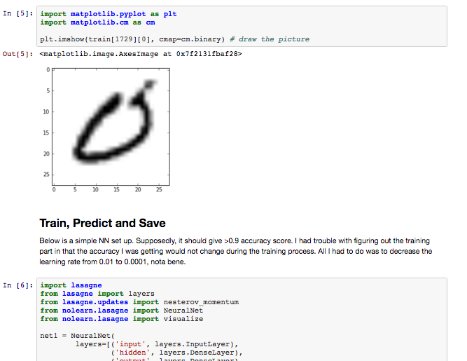
Kaggle tweeted my write up about Neural Networks and R.
Quick tutorial on using h2o for neural networks on the MSNIT Digit Recognizer dataset https://t.co/VnM3U0XVvQ pic.twitter.com/y9NRV5WPqP
— Kaggle (@kaggle) November 21, 2015